Adv. Macro – Ch. 2 Solow–Swan Cheatsheet

The Big Picture — What this model is trying to do

Core idea The whole story in three sentences

Countries are richer when they save more and invest more in machines. But machines have diminishing returns — the 1,000th machine added to a factory helps less than the 10th. This means every economy has a natural ceiling it gravitates toward, and once you hit it, you stop growing (unless technology improves).

The Solow model makes this precise. It takes three ingredients — a production function, a saving rule, and population growth — and shows that they always produce the same outcome: a unique stable resting point called the steady state, and a predictable path toward it called the transition.

Limitation What the model doesn't explain

In the steady state, output per worker is constant — it stops growing. But in real life, income per worker keeps rising (Kaldor fact K1). The model is a theory of levels, not long-run growth. The missing ingredient is technological progress, which Chapter 4 adds.

The saving rate $s$ is also just a fixed number — the model doesn't explain why people save what they save. That's fixed in Chapter 5.

What it's good for Three genuine predictions

1. Levels: Countries that invest more and grow more slowly in population should be richer. The data confirms both (correlations 0.59 and −0.66).

2. Conditional convergence: Countries grow faster when far from their own steady state. Also confirmed.

3. Great ratios: The capital–output ratio, factor shares, and return on capital should be roughly stable. Also confirmed — for now.

Variable Glossary — New in Chapter 2

Chapter 1 variables ($Y, N, \gamma, n, \pi, \ldots$) still apply. These are the new ones.

$k$

Capital per worker

$k_t = K_t / L_t$. The main state variable — everything in the model is driven by where $k$ is relative to $k^*$.

$y$

Output per worker

$y_t = Y_t / L_t = f(k_t)$. Since $L =$ population here, same as output per person.

$c$

Consumption per worker

$c_t = (1-s)y_t$. What people actually get to spend.

$f(k)$

Intensive production function

$y = f(k) \equiv F(k,1)$. The two-variable $F(K,L)$ reduced to one variable by dividing through by $L$.

$s$

Saving rate

Fraction of income saved/invested. Fixed parameter — the model's main weakness. $0 < s < 1$.

$\delta$

Depreciation rate

Fraction of capital that wears out each period. Typically $\delta \approx 0.05\text{–}0.10$.

$A$

Total factor productivity (TFP)

How efficiently inputs are converted to output. Fixed in Ch. 2; will grow in Ch. 4.

$\alpha$

Capital share / output elasticity

In Cobb–Douglas: share of income going to capital ($\approx 1/3$); also $\partial \log Y / \partial \log K$.

$k^*$

Steady-state capital per worker

The resting point where $s f(k^*) = (\delta+n)k^*$. Everything converges here.

$y^*, c^*$

Steady-state output and consumption

$y^* = f(k^*)$, $c^* = (1-s)y^*$. Constant once the economy arrives.

$\lambda$

Speed of convergence

$\lambda \approx (1-\alpha)(\delta+n)$. Fraction of the gap to $k^*$ closed each period. Different from Ch. 1's $\lambda_i$ welfare measure!

$r_t, w_t$

Rental rate of capital / wage

$r_t = f'(k_t)$, $w_t = f(k_t) - k_t f'(k_t)$. Appear only in the decentralized economy (Section 7).

$k_{GR}$

Golden-rule capital stock

The $k^*$ that maximizes steady-state consumption. Requires $s_{GR} = \alpha$. An economy above this is wastefully over-saving.

$\sigma$

Elasticity of substitution (CES)

How easily you can swap capital for labor. $\sigma = 1$ → Cobb–Douglas. $\sigma > 1$ → declining labor share as $k$ rises.

Part 1 — The Production Function

Concept Why divide everything by $L$?

The economy's output is $Y = F(K, L)$. But both $K$ and $L$ grow over time, which makes the math messy. The trick: because $F$ has constant returns to scale (doubling both inputs doubles output), you can divide everything by $L$ and get a single-variable problem:

$y = f(k)$ where $f(k) \equiv F(k, 1)$.

Now you just track capital per worker and everything else follows. This is called the intensive form.

Eq 6Cobb–Douglas production function

$$Y_t = A K_t^\alpha L_t^{1-\alpha}, \quad 0 < \alpha < 1$$ $$\text{Intensive form: } y = Ak^\alpha$$

What the parameters do: $A$ = TFP (how good the technology is). $\alpha$ = capital's share of income ($\approx 1/3$ in the data).

Think of it as: output = (quality of technology) × (machines)^⅓ × (workers)^⅔. If you double workers but keep machines fixed, output grows — but by less than double. That's diminishing returns.

Eq 7–8CES production function

$$Y = A\!\left(\alpha K^\gamma + (1-\alpha)L^\gamma\right)^{1/\gamma}, \quad \sigma = \frac{1}{1-\gamma}$$

The general version. Cobb–Douglas is the special case $\gamma \to 0$ ($\sigma = 1$).

The elasticity $\sigma$ tells you how flexible the economy is in substituting machines for workers. $\sigma = 1$ (Cobb–Douglas) → factor shares are constant no matter how much capital you accumulate. $\sigma > 1$ → as you add more capital, labor's share of income falls. This is the Karabarbounis–Neiman explanation for the declining labor share since 1980.

Eq 3–5Marginal products and Euler's theorem

$$F_K = f'(k), \qquad F_L = f(k) - k f'(k), \qquad F_K k + F_L = f(k)$$

MPK = slope of $f$. MPL = intercept of the tangent line to $f$ at $k$ (i.e. what workers would get per head). The last equation (Euler's theorem) says: pay every unit of capital its marginal product, pay every worker their marginal product, and the payments exactly add up to total output — zero profit left over. This is only possible under constant returns to scale.

A factory that pays fair market wages and fair rent on its machines breaks exactly even — no pure profit. This is why the model works: competitive markets and CRS together force profits to zero.

Part 2 — The Model: How Capital Evolves

Concept The core logic of capital accumulation

Each period, people save fraction $s$ of their income and invest it in new machines. At the same time, two things eat away at capital per worker: machines wear out (depreciation $\delta$) and new workers arrive each period (population growth $n$), each needing their share of machines. The economy's capital per worker rises only if new investment beats these two drains.

Eq 13–15The fundamental equation of the Solow model

$$(1+n)\,k_{t+1} = s f(k_t) + (1-\delta)k_t$$ $$\Downarrow \text{ rearranged (approximate)}$$ $$k_{t+1} - k_t \approx s f(k_t) - (\delta + n)k_t$$

Left side: change in capital per worker. Right side: new saving minus break-even investment. The term $(\delta + n)k_t$ is the break-even investment — the investment needed just to keep $k$ from falling. $\delta k_t$ replaces worn-out machines; $n k_t$ equips the new workers.

If $sf(k) > (\delta+n)k$: you're investing more than the drains, so $k$ rises next period. If $sf(k) < (\delta+n)k$: the drains win, $k$ falls. The steady state is where these exactly balance.

Part 3 — The Steady State

Concept What is a steady state and why does it always exist?

The steady state is the value $k^*$ where capital per worker stops changing — investment exactly offsets depreciation and population growth. Every economy with a neoclassical production function has exactly one such point, and it always ends up there from any starting point. Here's why:

The saving curve $sf(k)/k$ (saving per unit of capital) starts at $+\infty$ when $k\approx 0$ (because the first machine is enormously productive) and falls to zero as $k \to \infty$ (because of diminishing returns). The break-even line $\delta + n$ is flat. So the two must cross exactly once. Below the crossing, saving beats break-even → $k$ rises. Above, break-even beats saving → $k$ falls. The crossing is a magnet.

Eq 16, 18Steady-state condition and Cobb–Douglas solution

$$\text{General: } s f(k^*) = (\delta + n)k^*$$ $$\text{Cobb–Douglas: } k^* = \!\left(\frac{sA}{\delta+n}\right)^{\!\frac{1}{1-\alpha}}, \quad y^* = A^{\frac{1}{1-\alpha}}\!\left(\frac{s}{\delta+n}\right)^{\!\frac{\alpha}{1-\alpha}}, \quad \frac{K^*}{Y^*} = \frac{s}{\delta+n}$$

Read off from $y^*$: richer steady states come from higher $s$, lower $n$, lower $\delta$, or higher $A$. Three key elasticities:

Income w.r.t. saving rate: $\partial \log y^* / \partial \log s = \alpha/(1-\alpha) = 1/2$ for $\alpha=1/3$. Doubling $s$ raises $y^*$ by 41%, not 100%.
Income w.r.t. $\delta+n$: same magnitude, opposite sign.
Income w.r.t. TFP $A$: $1/(1-\alpha) = 3/2$. A productivity advantage is amplified by the extra capital it induces.

The capital–output ratio $K^*/Y^* = s/(\delta+n)$ is just saving rate over break-even. With $s=0.2$ and $\delta+n=0.06$, you get $\approx 3.3$ — matching Kaldor's K4.

The Solow Diagram — Reading it

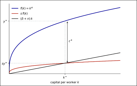
Reading the diagram: The steady state $k^*$ is where the red saving curve $sf(k)$ crosses the black break-even ray $(\delta+n)k$. At that point, $y^*$ is the height of the blue output curve, $sy^*$ is the height of the crossing, and the gap between them is steady-state consumption $c^*$.

To the left of $k^*$: saving > break-even → $k$ rises. To the right: break-even > saving → $k$ falls. The steady state is stable from both sides.

Comparative statics: Higher $s$ rotates the saving curve up → $k^*$ moves right (richer). Higher $n$ or $\delta$ steepens the ray → $k^*$ moves left (poorer). Higher $A$ shifts both curves up → richer. In all cases, only the level changes, never the long-run growth rate.

Part 4 — Transition Dynamics: Getting to the Steady State

Concept How fast does the economy grow along the way?

If a country is far below its steady state (say, just after a war destroyed its capital stock), it will grow fast. As it gets closer to $k^*$, growth slows down and asymptotes to zero. This is because of diminishing returns: the further below $k^*$ you are, the higher the marginal product of capital, so each unit of saving buys more growth.

Important: growth is fast relative to your own steady state. A poor country with a low $k^*$ near its ceiling doesn't necessarily grow faster than a rich country that's far from its high ceiling.

Eq 20–22Growth rate along the transition

$$\gamma_{k,t} = sAk_t^{\alpha-1} - (\delta+n)$$ $$\gamma_{y,t} \approx \alpha\!\left(sA^{1/\alpha} y_t^{-\frac{1-\alpha}{\alpha}} - \delta - n\right)$$

Growth of capital (and output) is a decreasing function of the current level. The further below $k^*$, the higher the average product of capital, the more growth you get per unit of saving.

When $k$ is tiny, even a small amount of saving buys a lot of growth because the marginal machine is hugely productive. As you accumulate more capital, each additional machine helps less and less, so growth slows — until it hits zero at $k^*$.

Eq 23Speed of convergence $\lambda$

$$\log k_{t+1} - \log k^* \approx (1-\lambda)\left(\log k_t - \log k^*\right)$$ $$\lambda \approx (1-\alpha)(\delta + n)$$ $$\text{Half-life: } t_{1/2} \approx \frac{\log 2}{\lambda}$$

Each period, the economy closes fraction $\lambda$ of its log-distance to the steady state. With $\alpha=1/3, \delta=0.05, n=0.01$: $\lambda \approx 0.04$ and the half-life is 17 years.

Why is the data slower? Barro and Sala-i-Martin find $\lambda \approx 0.02$ (half-life 35 years) in regional data. The Solow model converges twice as fast. The fix: add human capital (Ch. 4), which effectively raises $\alpha$ to $\approx 2/3$ and halves $\lambda$.

Concept Conditional vs. Unconditional Convergence — the key distinction

What the model actually predicts is conditional convergence: for a given set of parameters $(s, n, \delta, A)$, a poorer country (lower $k$ relative to its own $k^*$) grows faster. If two countries have identical parameters, the poorer one will catch up.

What it does NOT predict is unconditional convergence: the model says nothing about whether a randomly selected poor country (which may have a lower $k^*$ due to bad policies, low saving, or fast population growth) should grow faster than a randomly selected rich country.

So: observing that poor countries don't on average grow faster than rich ones is not evidence against Solow — it just means their steady states differ. The data actually supports conditional convergence strongly ($\beta \approx 0.01\text{–}0.02$), and since about 2000 even unconditional convergence has appeared, because poor-country fundamentals (education, institutions) have improved enough to make steady states converge.

Part 5 — The Golden Rule and Dynamic Inefficiency

Concept What saving rate makes people happiest?

Different saving rates give different steady states with different consumption levels. The golden-rule saving rate is the one that maximizes steady-state consumption $c^* = f(k^*) - (\delta+n)k^*$. It turns out to be $s_{GR} = \alpha$: exactly equal to the capital share.

If a country saves more than $\alpha$ (i.e. $s > \alpha$), it's dynamically inefficient: people are over-investing. They could consume more at every date — now and in the future — simply by saving less. Nobody would choose this if they cared about consumption. The fact that this is possible at all is a sign that the model's fixed saving rule is a weakness (Chapter 5 fixes this with optimization).

For the record, the US saves about 20% while $\alpha \approx 1/3$, so $s < \alpha$ — the US is not dynamically inefficient.

Eq 24–26Golden rule conditions

$$c^* = f(k^*) - (\delta+n)k^*$$ $$f'(k_{GR}) = \delta + n \quad \Longrightarrow \quad s_{GR} = \alpha$$

Maximize $c^*$ over $k^*$: the golden-rule condition says the marginal product of capital should equal break-even investment. In the Cobb–Douglas case this simplifies neatly to saving rate = capital share.

In the Solow diagram, $c^*$ is the vertical gap between $f(k)$ and the ray $(\delta+n)k$. This gap is widest where the tangent to $f(k)$ is parallel to the ray — i.e., where $f'(k) = \delta+n$.

Modified golden rule Ch. 5 preview

When households optimize (Chapter 5), the optimal path satisfies a modified golden rule: $f'(k) = \delta + n + \rho$, where $\rho$ is the household's rate of time preference (impatience). Because $\rho > 0$, the optimal $k$ is below the golden rule — patient investment pays off but impatient people don't over-save. Dynamic inefficiency ($s > \alpha$) can't arise when people optimize.

Part 6 — The Decentralized Economy (Markets give the same answer)

Concept Why bother with firms and households separately?

So far the model was run by a planner who just applies the saving rule. But real economies have firms renting capital and hiring labor, and households owning the factors and choosing how much to save. The key result: competitive markets produce exactly the same aggregate path as the planner. This matters because it shows the Solow model is a valid description of actual market economies, not just a planning exercise. It also tells us the prices — wages and returns — which the planner's problem never mentions.

Eq 27–29Factor prices and shares in equilibrium

$$r_t = f'(k_t) = \alpha k_t^{\alpha-1}, \qquad w_t = f(k_t) - k_t f'(k_t) = (1-\alpha)k_t^\alpha$$ $$\frac{w_t L_t}{Y_t} = 1-\alpha, \qquad \frac{r_t K_t}{Y_t} = \alpha$$

Firms set marginal product = price. In equilibrium all firms choose the same capital–labor ratio (the aggregate ratio), so the economy behaves like one big firm. Factor shares are constant at every date — this is Kaldor fact K5, but in Cobb–Douglas it's assumed by the functional form, not derived.

Each machine earns its marginal product $r$, each worker earns their marginal product $w$, and by Euler's theorem these payments add up to exactly 100% of output — no profit left. Capital gets $\alpha \approx 33\%$, labor gets $1-\alpha \approx 67\%$, always.

Part 7 — Confronting the Data

Eq 33–34Lucas's puzzle: why doesn't capital flow to poor countries?

$$\frac{y_R}{y_P} = \left(\frac{s_R}{s_P}\right)^{\!\frac{\alpha}{1-\alpha}} \Rightarrow \frac{s_R}{s_P} = \left(\frac{y_R}{y_P}\right)^{\!\frac{1-\alpha}{\alpha}} = 12^2 = 144$$ $$\frac{r_P}{r_R} = \left(\frac{y_R}{y_P}\right)^{\!\frac{1-\alpha}{\alpha}} = 144$$

If the US–India income gap (12×) is entirely due to different capital stocks, the return on capital in India would need to be 144× higher than in the US. That would attract every dollar of capital in the world to poor countries instantly. But it doesn't happen.

The reductio: the premise (income gaps = capital gaps alone) is impossible. Either (a) capital broadly defined includes human capital → raise $\alpha$ to 2/3 and the ratio drops to 12^0.5 = 3.5, plausible; or (b) TFP $A$ differs across countries — poor countries just have worse technology. Option (b) is probably the main answer, which motivates Chapters 6–7.

Eq 35–36$\beta$- and $\sigma$-convergence

$$\frac{1}{T}(\log y_{i,T} - \log y_{i,0}) = a + b\log y_{i,0} + \varepsilon_i$$ $$\sigma^2_T = (1+bT)^2 \sigma^2_0 + T^2\sigma^2_\varepsilon$$

$\beta$-convergence: $b < 0$ means poorer countries grow faster (conditional or unconditional). $\sigma$-convergence: the cross-country dispersion of log income is falling.

Key asymmetry: $\beta$-convergence is necessary but not sufficient for $\sigma$-convergence — if idiosyncratic shocks ($\sigma_\varepsilon$) are large enough, dispersion can widen even while poor countries on average catch up. Also: $b < 0$ can be spurious (Galton's fallacy with measurement error). That's why both concepts matter together.

Convergence Evidence: What the Data Says

Finding	Period	Result	Consistent with Solow?
Unconditional convergence	1960–1990	Slope $b \approx +0.28$ — divergence	conditional only Steady states differ; Solow only predicts conditional
Unconditional convergence	1990–2023	Slope $b \approx -0.14$ — weak convergence	yes Poor-country fundamentals (education, institutions) converged → steady states now more alike
Conditional convergence	1960–present	$\beta \approx 0.01\text{–}0.02$ throughout	yes Robust, present throughout the entire post-war period
$\sigma$-convergence (unweighted)	1960–2023	Dispersion rose through 2000, slightly fell after	consistent Small $b$ + large idiosyncratic shocks → Eq (36) predicts exactly this
$\sigma$-convergence (population-weighted)	Post-1990	Fell sharply (China, India)	yes Most populous countries caught up
Speed of convergence $\lambda$	Regional data	Estimated $\lambda \approx 0.02$ (half-life 35 yr)	too slow Solow predicts $\lambda \approx 0.04$. Fix: add human capital → Ch. 4

Model Scorecard

Gets right ✓

✓ Capital–output ratio $\approx 3\text{–}4$ (Kaldor K4)

✓ Constant factor shares (K5, by assumption in CD)

✓ Constant return on capital (K3)

✓ Higher investment → higher income (corr 0.59)

✓ Higher pop growth → lower income (corr −0.66)

✓ Conditional convergence exists and is stable

Gets wrong ✗

✗ No long-run growth — violates Kaldor K1

✗ Convergence speed too fast ($\lambda$ 2× data)

✗ Income gaps too big for capital differences alone (Lucas puzzle)

✗ Saving rate $s$ unexplained — just a parameter

✗ Can't explain why TFP $A$ differs across countries

Next chapters fix

→ Ch. 4: Add tech progress ($A$ growing) and human capital. Fixes growth, improves convergence speed.

→ Ch. 5: Replace fixed $s$ with household optimization. Fixes dynamic inefficiency.

→ Ch. 6–7: Explain where $A$ comes from (endogenous growth).

Formula Quick Reference

Eq 17Growth rate of capital (transition)

$$\gamma_{k,t} = s\frac{f(k_t)}{k_t} - (\delta + n)$$

Saving per unit of capital minus break-even. Positive below $k^*$, zero at $k^*$, negative above.

Eq 19Elasticity of $y^*$ with respect to $s$

$$\frac{\partial \log y^*}{\partial \log s} = \frac{\alpha}{1-\alpha}$$

For $\alpha=1/3$: doubling $s$ raises $y^*$ by $2^{1/2}-1 \approx 41\%$. Same elasticity (negative) for $\delta+n$. Elasticity w.r.t. $A$ is $1/(1-\alpha) = 3/2$.

Eq 23Log-linear convergence

$$\log k_t - \log k^* \approx (1-\lambda)^t (\log k_0 - \log k^*)$$ $$\lambda \approx (1-\alpha)(\delta + n), \quad t_{1/2} \approx \frac{\log 2}{\lambda}$$

Each period closes fraction $\lambda$ of the gap. With tech progress add $\gamma_A$: $\lambda = (1-\alpha)(\delta+n+\gamma_A)$.

Eq 32Steady-state prices and ratios

$$r^* = \alpha\frac{\delta+n}{s}, \quad \frac{K^*}{Y^*} = \frac{s}{\delta+n}, \quad \frac{wL}{Y}=1-\alpha, \quad \frac{rK}{Y}=\alpha$$

All four are constant in steady state → Kaldor facts K3, K4, K5. With $\alpha=1/3, s=0.2, \delta+n=0.06$: $K/Y = 3.3$, $r^* \approx 10\%$ gross.

Chapter 2 · Advanced Macroeconomics · University of Ljubljana · Oct 2026

Advanced Macroeconomics — Chapter 2: The Solow–Swan Model